Verification Cases:
Several verification cases are provided below to demonstrate the accuracy and efficiency of the FastBEM Acoustics® software. Cases with different types of domains (exterior or interior), acoustic sources (radiation or scattering), and boundary conditions (pressure, velocity, or impedance) are presented. Other verification cases can be found in the User Guide or the book and papers listed on the References page (To view larger and better-quality plots or videos, click on the images).
Download the Verification Manual.
A. Radiation from A Vibrating Sphere
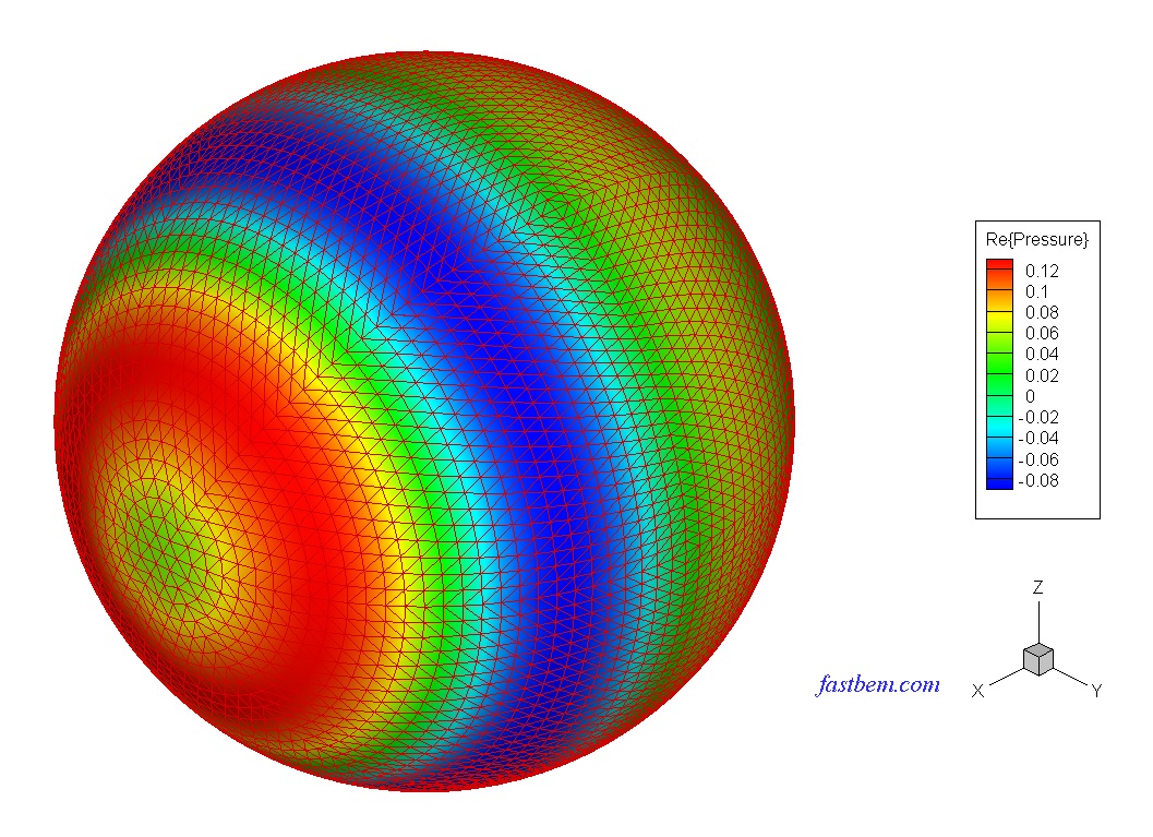
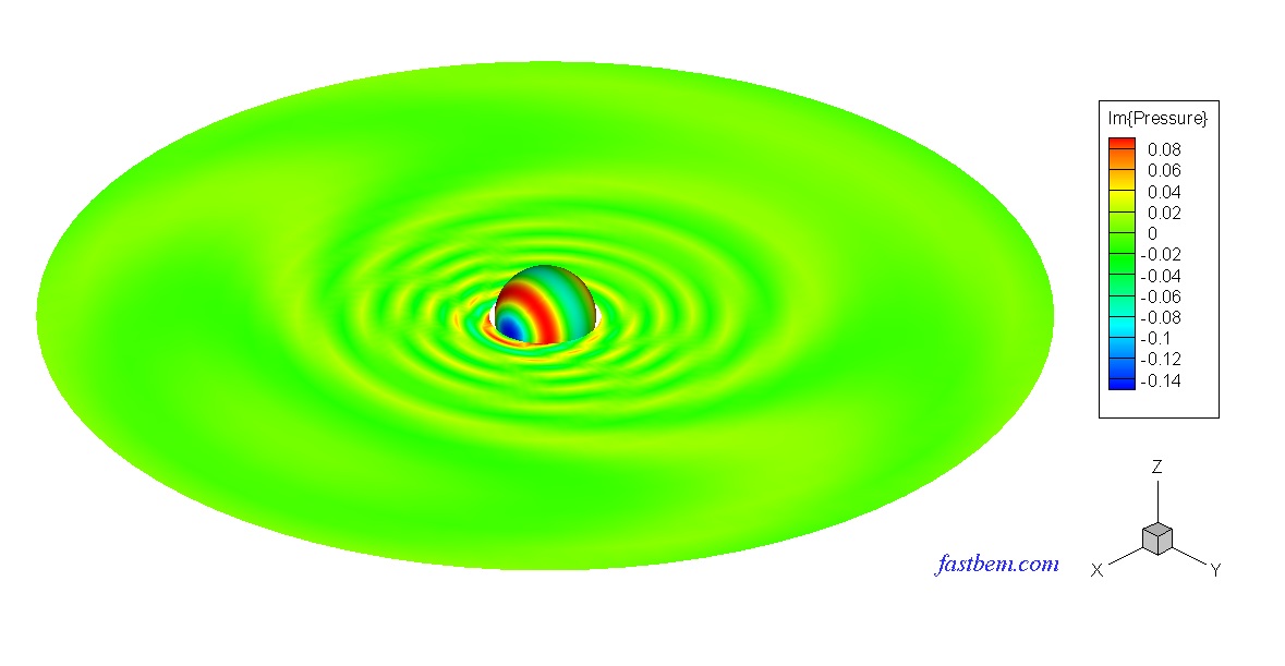
The sound field outside a vibrating sphere of radius R (=1) is studied in this case. To make the field nonuniform on the boundary, a monopole source is placed at the off-center location (R/2, 0, 0) to generate the velocity BCs on the boundary of the sphere and the exterior field is solved using the software. The number of elements increases from 588 to 4,320,000. The nondimensional wavenumber ka = 2 or 20. The following two contour plots show the sound pressure on the surface of the sphere and a field surface, respectively, at ka = 20 and with 10,800 elements (Click on the images to see larger plots).
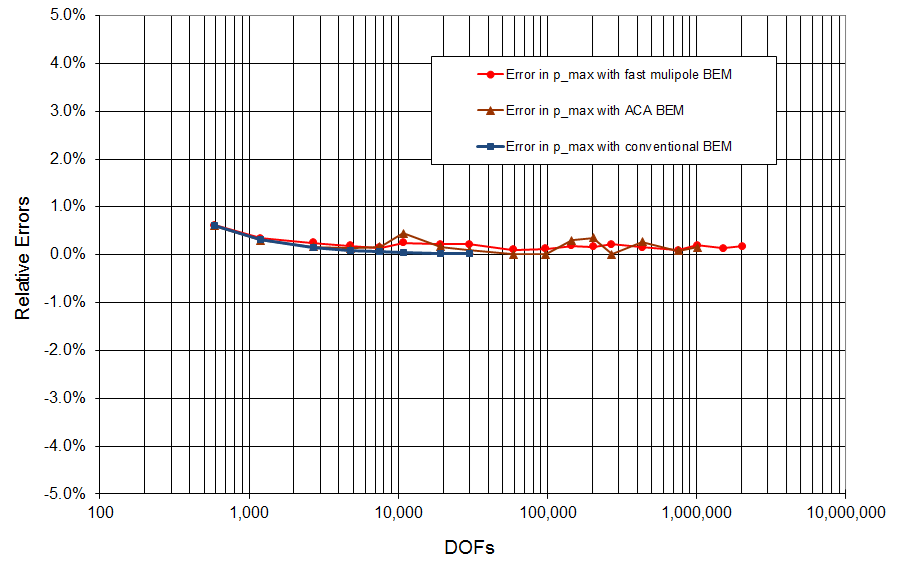
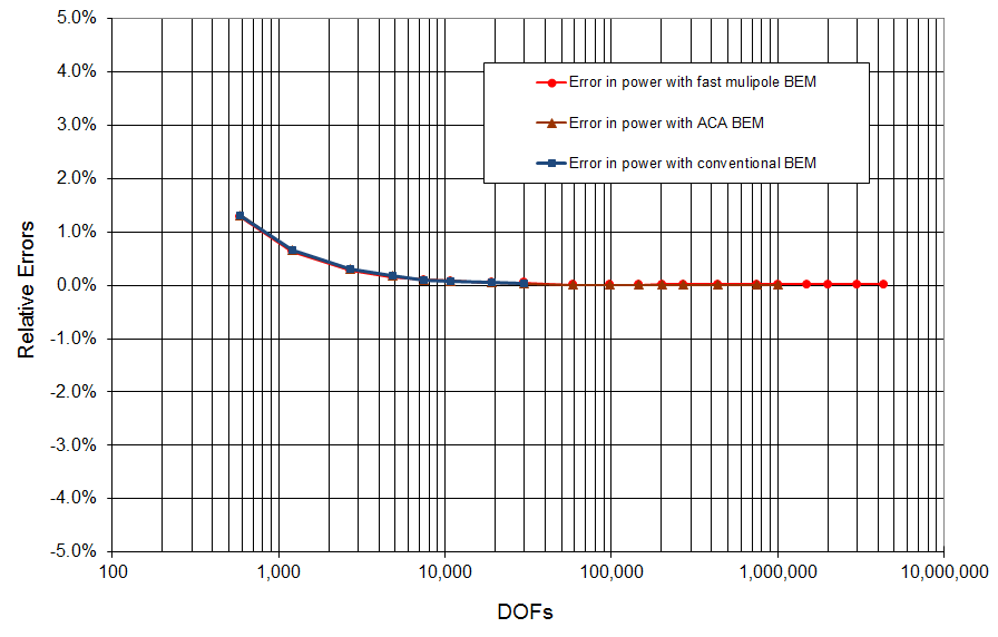
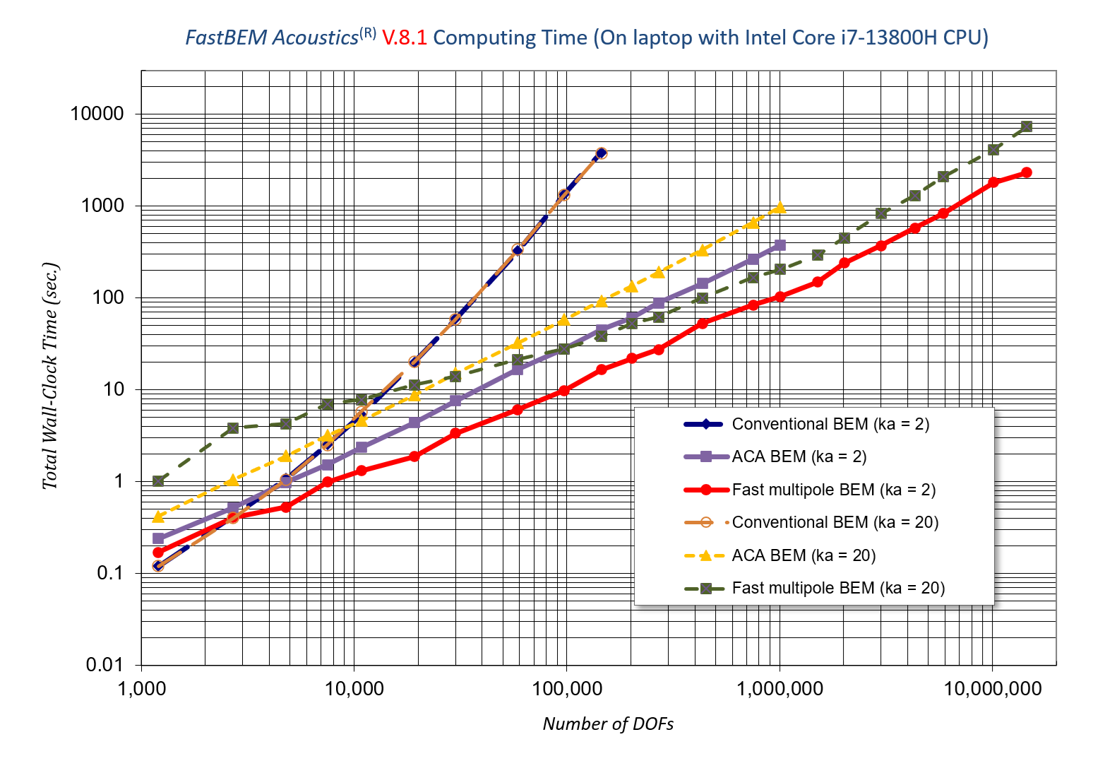
Plots of relative errors in the computed sound pressure and power, and plot of the total wall-clock time are shown in the following three plots, respectively. The accuracy of the FastBEM Acoustics® is very satisfactory with the errors decreasing quickly and staying around 0.3% for models with more than 100,000 DOFs at ka = 2, indicating the numerical stability of the algorithms. The solution time for the FastBEM Acoustics® code with the fast multipole BEM solver increases almost linearly with the increase of the DOFs and the largest BEM model with 5.88 million DOFs is solved in 15 min. at ka = 2, and in 20 min. at ka = 20 (using 4 threads out of 20 on a laptop with Intel® Core i7 13800-H CPU). The conventional BEM can solve BEM models with up to 145,200 DOFs and the solution time used increases almost as a cubic function of the DOFs. The adaptive cross approximation (ACA) BEM solver is also very efficient in solving BEM models with up to 1,000,000 DOFs in this case.
B. Radiation from A Transversely Oscillating Sphere
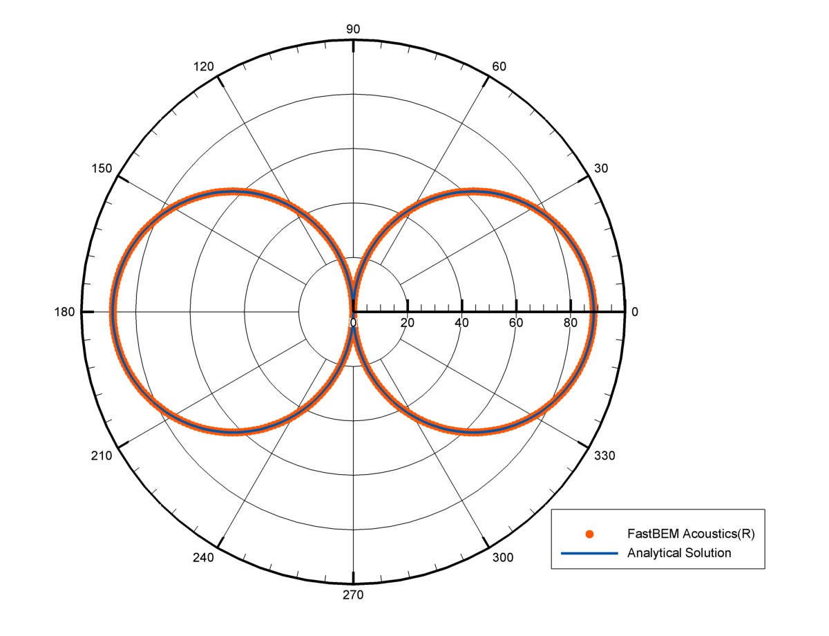
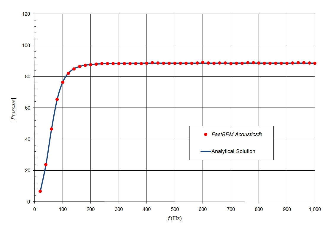
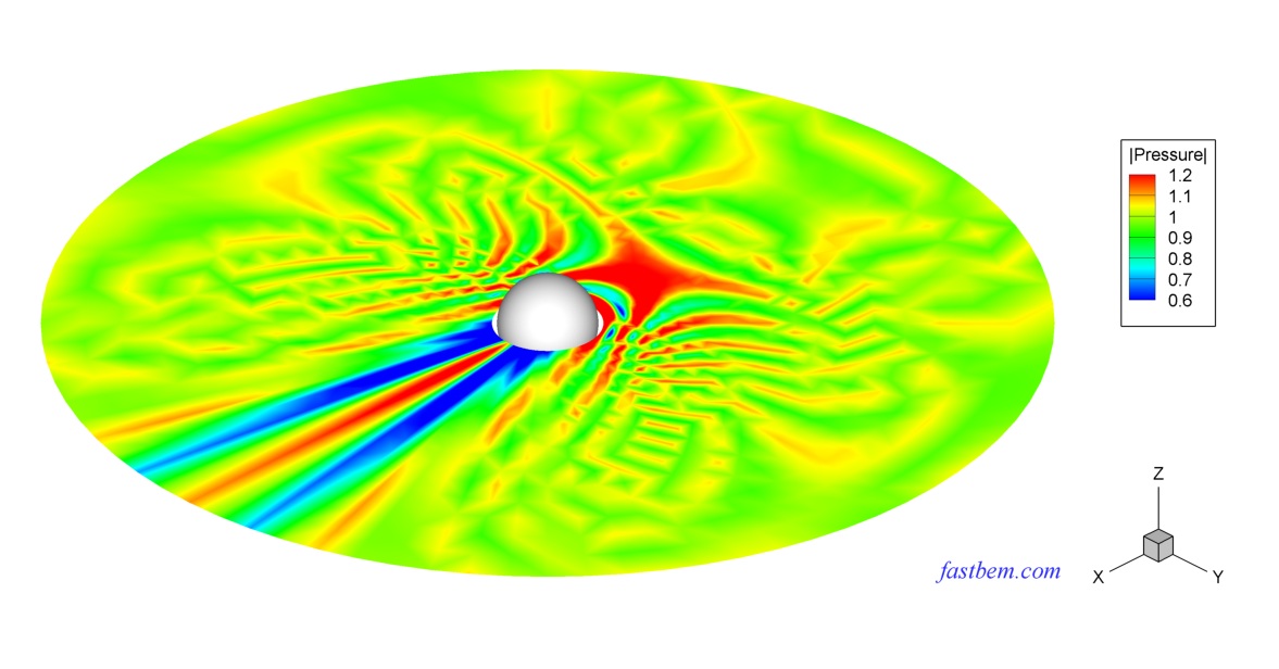
The sound field radiated from an oscillating sphere of radius R (=1) is considered in this case. The sphere is oscillating in the x-direction and 30,000 elements are used in the mesh. The first picture below is a video that shows the radiated sound pressure field outside the sphere at f = 500 Hz. The second figure shows the angular distribution of the sound pressure along a circle of radius 5R and compared with the analytical solution at this frequency. The last figure shows the pressure values at the point (5R, 0, 0) in the frequency range of 20-1000 Hz (where ka = 36.62) and compared with the analytical solution. The dual BIE option and fast multipole BEM solver are used in this case, which is an exterior acoustic wave problem and the dual BIE option can remove the fictitious eigenfrequencies. Another frequency sweep example for a pulsating sphere can be found in the User Guide.
C. Field Inside A Vibrating Sphere
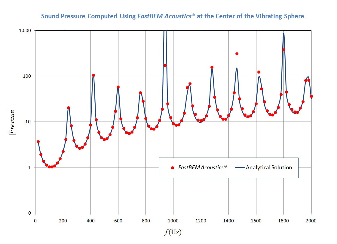
The sound field inside a vibrating sphere of radius R is considered in this case. A velocity of constant amplitude is specified on the boundary of the sphere and the sound pressure at the center of the sphere is computed for frequencies from 20 Hz to 2000 Hz (where ka = 73.24). Two boundary element meshes are used, one with 30,000 elements for calculations with frequencies up to 1360 Hz, and another mesh with 58,800 elements for other frequencies up to 2000 Hz. The fast multipole BEM solver is used in this case. The following plot shows the computed sound pressure at the center of the sphere as compared with the analytical solution. The peaks are near the resonant frequencies of the medium where the values tend to infinity theoretically.
D. Scattering from A Rigid Sphere
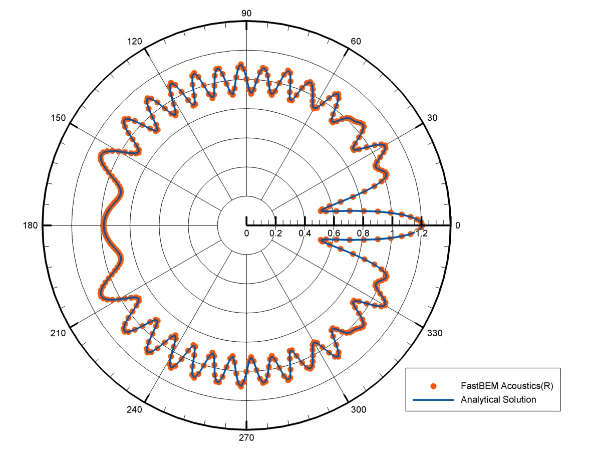
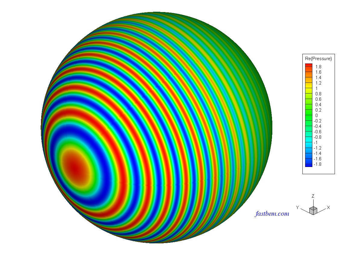
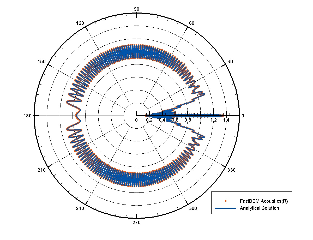
In this case, the sound field from a rigid sphere of radius R and impinged upon by a plane incident wave is computed using the software and the results are verified with the analytical solution. The incident wave is in the +x direction. A total of 10,800 elements are used in the mesh and the nondimensional wavenumber ka = 20. The fast multipole BEM solver is used. The first figure in the following shows a contour plot of the computed sound pressure on a field surface with an outer radius of 10R. The second figure shows a polar plot of the computed sound pressure at the points on this field surface along a circle of radius 5R and compared with the analytical solution. The maximum error in the BEM results is 0.18% for this plot.
![]()
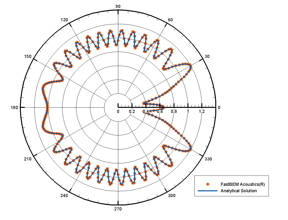
The same case is tested at a higher frequency of ka = 100 (f = 2730 Hz), using a finer mesh with 187,500 elements. The ACA BEM solver is used. The first figure in the following shows a contour plot of the computed sound pressure on the surface of the sphere. The second figure shows a polar plot of the computed sound pressure at the points along a circle of radius 5R and compared with the analytical solution. The maximum error in the BEM results is 3.21% for this plot.
E. Scattering from A Soft Sphere
This case is identical to the one discussed above (with ka = 20), except that the boundary condition is changed to zero pressure condition (a soft sphere). The first figure in the following shows a contour plot of the computed sound pressure on the field surface. The second figure shows a polar plot of the computed sound pressure at the points along a circle of radius 5R and compared with the analytical solution. The maximum error in the BEM results is 0.45% for this plot.

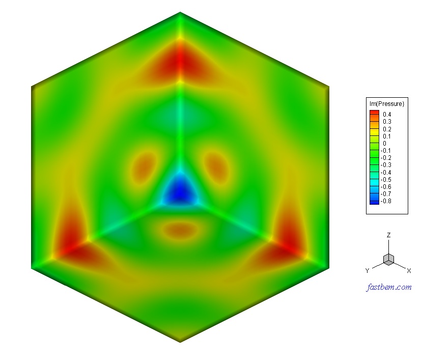
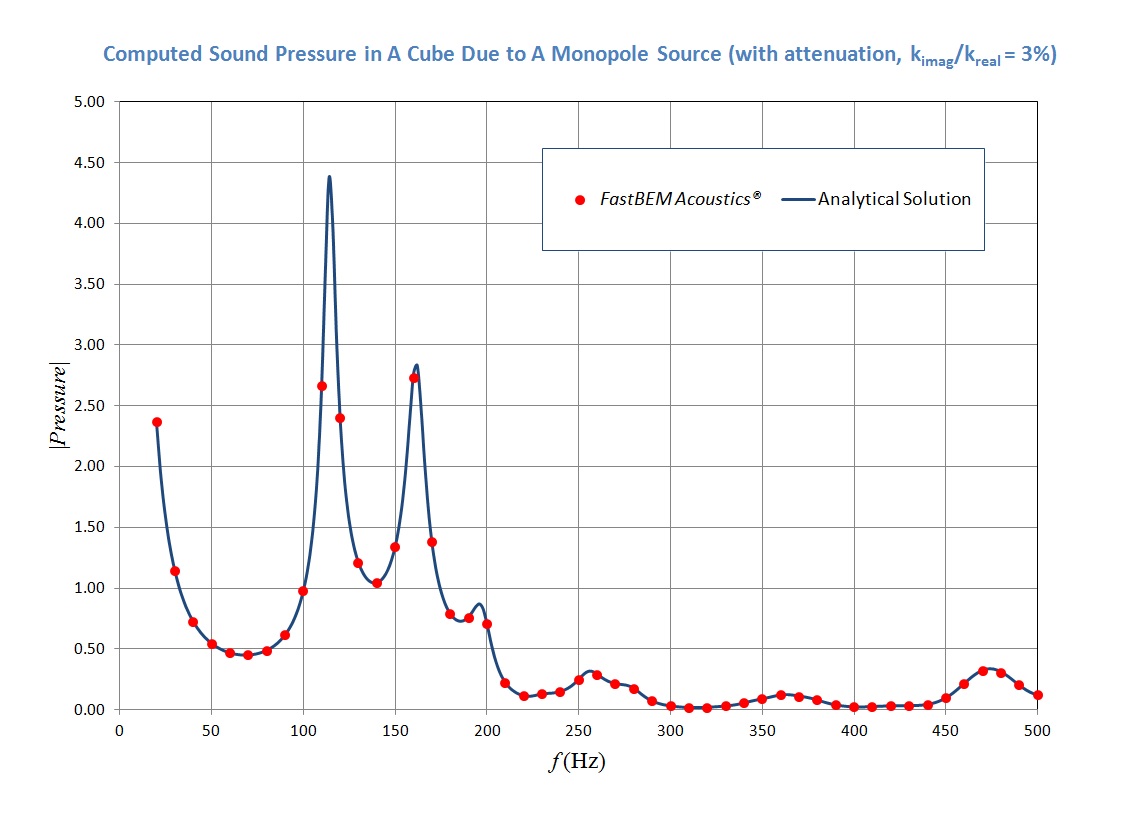
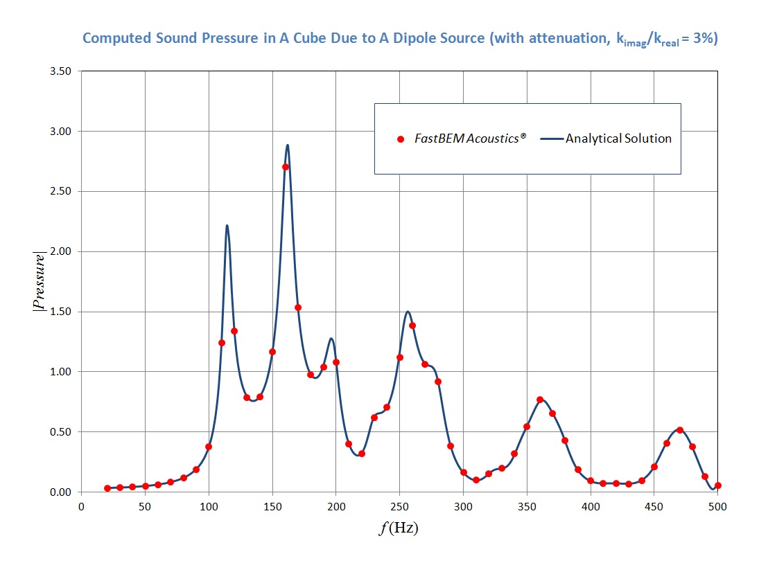
F. Sound from Monopole and Dipole Sources
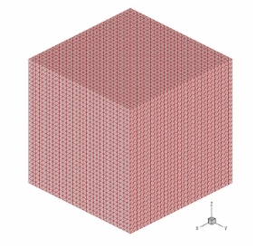
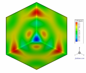
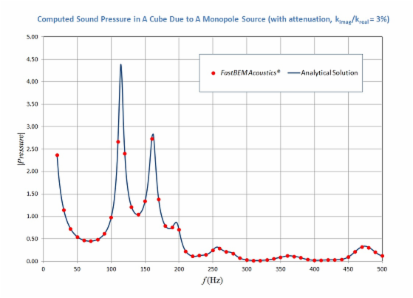
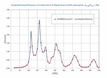
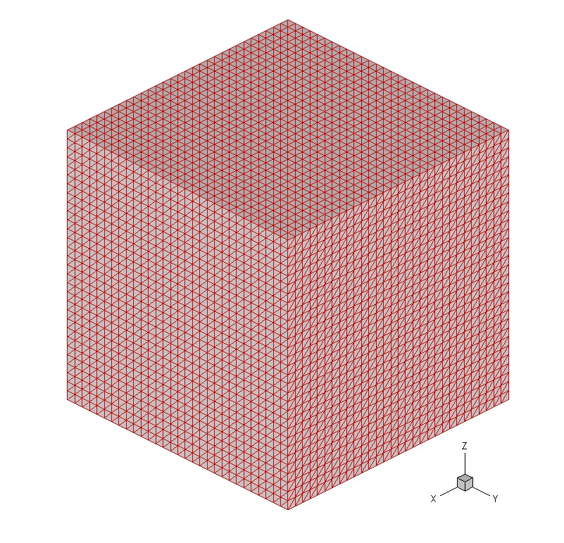
The sound field in a cube of dimensions 1.5 m X 1.5 m X 1.5 m is modeled to verify the BEM results using monopole and dipole point sources. The walls of the cube are considered rigid. The point source (monopole or dipole) is placed at the location (0.3, 0.3, 0.3) m and a field point is placed at (1.2, 1.2, 1.2) m. A total of 10,800 elements are used in the BEM model. The acoustic pressure at the field point is computed between f = 20-500 Hz for two situations, one with the monopole source and the other with the dipole source. To reduce the peaks at the resonance frequencies of the medium inside the cube, a small attenuation or damping effect is introduced in the solutions by using a complex wavenumber k in this case (Applying a complex wavenumber is available in the new release FastBEM Acoustics® V.3.0.0). The BEM results are compared with the analytical solutions [A. Pierce, Acoustics, ASA, 1991]. In the following, the first two pictures show the mesh for the cube and the computed pressure on the surface of the cube due to the monopole source and at f = 500 Hz. The two plots show the pressure at the field point due to the monopole and dipole source, respectively. Good agreements of the BEM results with the analytical solutions are observed.
G. Sound in A Vibrating Box Channel
A box channel of dimensions 2 m X 0.5 m X 0.5 m is modeled here. This is an interior domain problem. Velocity boundary conditions corresponding to a plane wave travelling in the x-direction are applied at the two ends of the channel. The lateral surfaces are applied with zero velocity (rigid) boundary conditions. A total of 51,600 elements are used in the BEM model. The acoustic pressure on the surfaces of the channel and at the field points along the long axis of the channel are computed at ka = 100 (f = 2730 Hz). The model is solved with the ACA BEM solver. The computed acoustic pressure on the surfaces of the channel and at the field points along its axis are shown in the following video and plot, respectively. The maximum error in the BEM results is less than 2% as compared with the analytical solution.

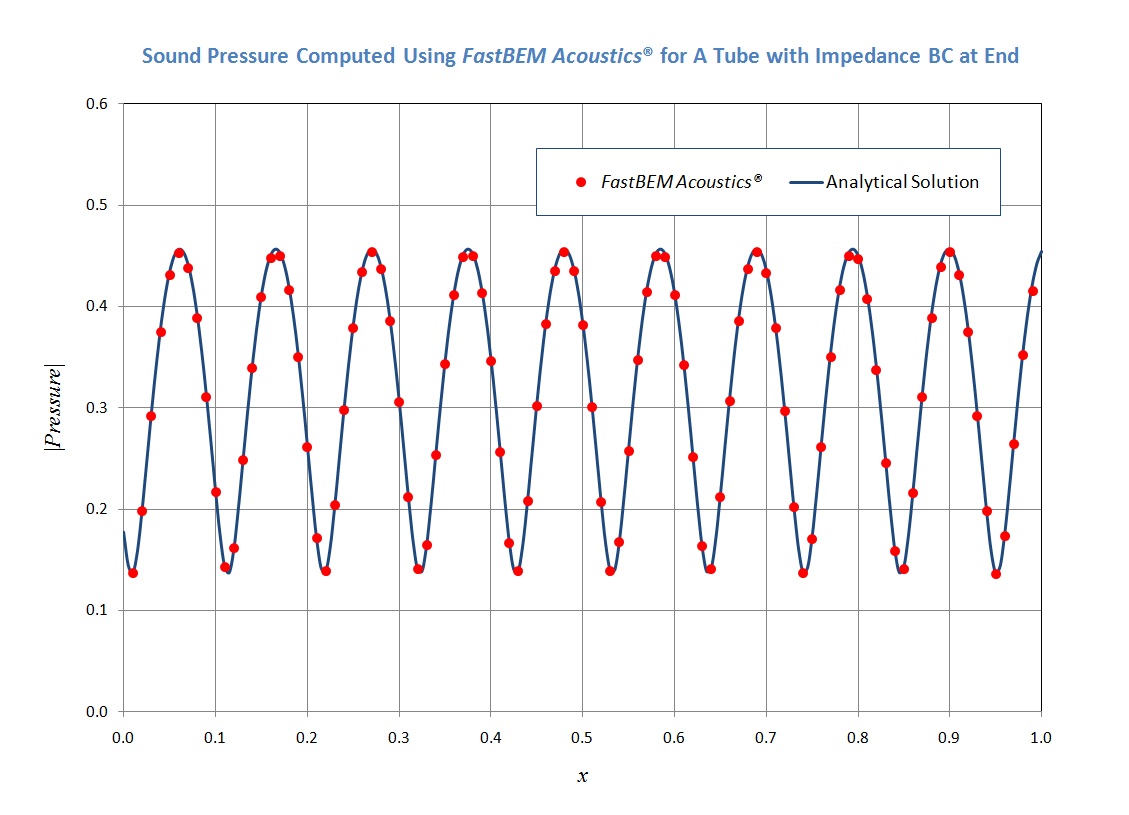
H. A Tube with Impedance Boundary Condition at End
A tube of dimensions 1 m X 0.1 m X 0.1 m and with an impedance boundary condition is modeled in this case. The side walls of the tube are rigid. The end at x = 0 is applied with a velocity of 0.001 m/s, while the end at x = 1 m is applied with an impedance Z = (3, 1)ρc. A total of 8400 elements are used in the BEM model and the frequency is at f = 1638 Hz (ka = 30). The model is solved with the fast multipole BEM solver. The computed acoustic pressure on the surfaces of the tube and at the field points along the axis are shown in the following video and plot, respectively. The maximum error in the result on the plot is 1.85% as compared with the analytical solution [A. Pierce, Acoustics, ASA, 1991].
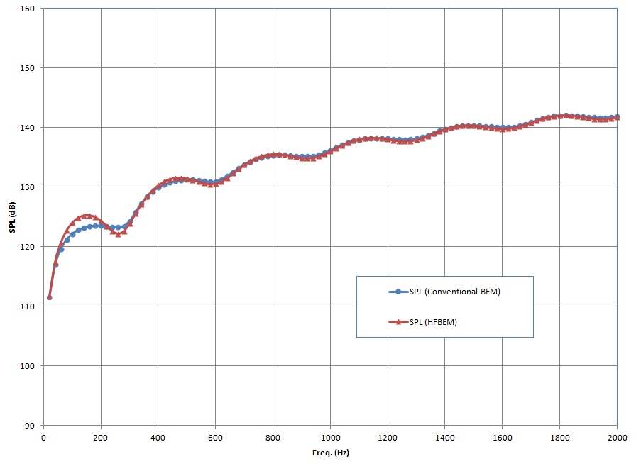
I. Radiation from A Box Using the HFBEM
The sound field outside a radiating box with dimensions 1 m X 1 m X 1 m is modeled in this case. The six surfaces of the box are applied with a velocity of 1 m/s. A total of 1200 elements are used in the BEM model and the frequency is from 20 Hz to 2000 Hz. The model is solved with the conventional BEM solver and the high-frequency BEM (HFBEM) option (See the User Guide for the formulation used in the HFBEM). The plot below shows the computed sound pressure level (SPL) at the field point (10 m, 0, 0). It is shown that the HFBEM is quite accurate for estimating the far field sound pressure field, especially at the higher frequencies. In this case, the total CPU time used with the HFBEM is less than 1% of that used with the conventional BEM, which clearly demonstrates the usefulness of the HFBEM in solving exterior radiation problems at the high frequencies.